Carlos CB
MSc thesis
Here I show what I worked on for my MSc and my BSc thesis (source code available). Both are presented here as a single thing, but in reality the work was incremental and one continued where the other left off. This work was originally presented in July of 2019.
In this page, although abridged, almost everything presented in my MSc thesis is included, and it’s quite a lot of text. I would recommend reading (or skimming) the abstract and then heading to the experimental results and conclusions sections to get a general sense of the work.
If you’re interested and want to learn more about ordinal classification and how it was treated in this particular work, then head to the that particular section.
Table of contents
Comparative Study of Different Loss Functions for Deep Neural Networks on Ordinal Classification Problems
Abstract
This work was a new approach for ordinal classification problems using deep learning models. It is based on the use of ordinal loss functions and unimodal probability density functions. The use of unimodal probability distributions is based on the work of Beckham et al., and it works by transforming the output distribution given by a deep neural network into an unimodal distribution. With this set up, during the training process the distance between classes isn’t used to calculate the errors in the predictions made by the model and so the weights aren’t modify accordingly; the ordinality is only considered in the last layer. This approach was improved by adding new ordinal loss functions that use the ordinal information inherent to the labels during the training process to modify the network’s weights.
With this approach, we present a comparative study of the results obtained when:
- A regular non-ordinal loss function, cross entropy, is used on a baseline non-ordinal model
- A model that takes into account the ordinality only by using unimodal probability density functions
- Different ordinal loss functions are used in conjunction with unimodal probability distributions for the network output
For the comparison, an ordinal dataset is considered, Adience, which contains images of faces with a label indicating a range of ages for the person in the picture. This is the label used for training. To put it briefly, the ordinality in the labels comes from the error being greater when misclassifying a baby (class 0) for a grown man (class 4) than when misclassifying that same baby as a toddler (class 1); or the error being smaller when mistaking an senior (class 5) with an elder (class 6) than with a teenager (class 3). So in ordinal classification these greater errors are penalized with a bigger cost than smaller errors. The difference between labels is also called distance, further labels (baby vs adult) have a greater distance than closer labels (baby vs toddler). The cost of misclassification is calculated with the distance between classes.
For this study we selected two loss functions previously presented in the literature: QWK, Quadratic Weighted Kappa, and EMD, Earth Mover’s Distance; and made a new proposal, an ordinal loss function based on the MSE, Mean Squared Error. For this proposed loss function two alternatives are derived depending on the weighting of the costs, one with an absolute value weighting, named wMSE, meaning Weighted MSE, and another one with a quadratic weighting, qMSE, which stands for Quadratic Weighted MSE.
The results obtained show that using ordinal loss functions improves the base results obtained in other works that used the same dataset, and also considerably improves the baseline models used on this study. We also conclude from the results that the quadratic weighting in the cost of misclassification improves an absolute weighting.
(If you are just looking over, I would recommend skipping to experimental results.)
Ordinal Classification
Ordinal classification is a ML task which tackles a problem where there is an inherent order in the classes to predict. The goal is to leverage the information given by the ordering of the classes to improve the training and inference when new samples are presented. The main trait that sets it apart from nominal (normal) classification is that the misclassification error is not the same among any pair of classes, the error increases with the distance among classes.
The common characteristics to any ordinal classification problem are:
- Discreet classes
- Natural order
Some examples of ordinal classification are:
- Predicting the severity of a disease
- Ranking or preference prediction
- Exam grades
- Credit score
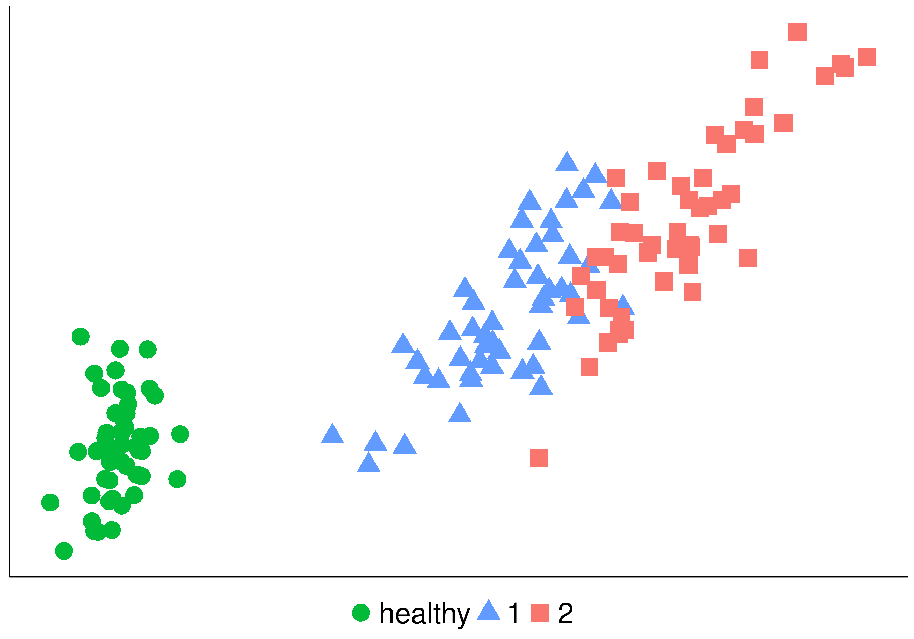
In the following figure you can see the same problem treated as a nominal and ordinal classification problem. On the left we have two classes, healthy, or ill. If we transform the problem adding ordinality, the we have: healthy, and in the ill class we have degree 1 or 2 indicating the severity.
| Nominal | Ordinal |
|---|---|
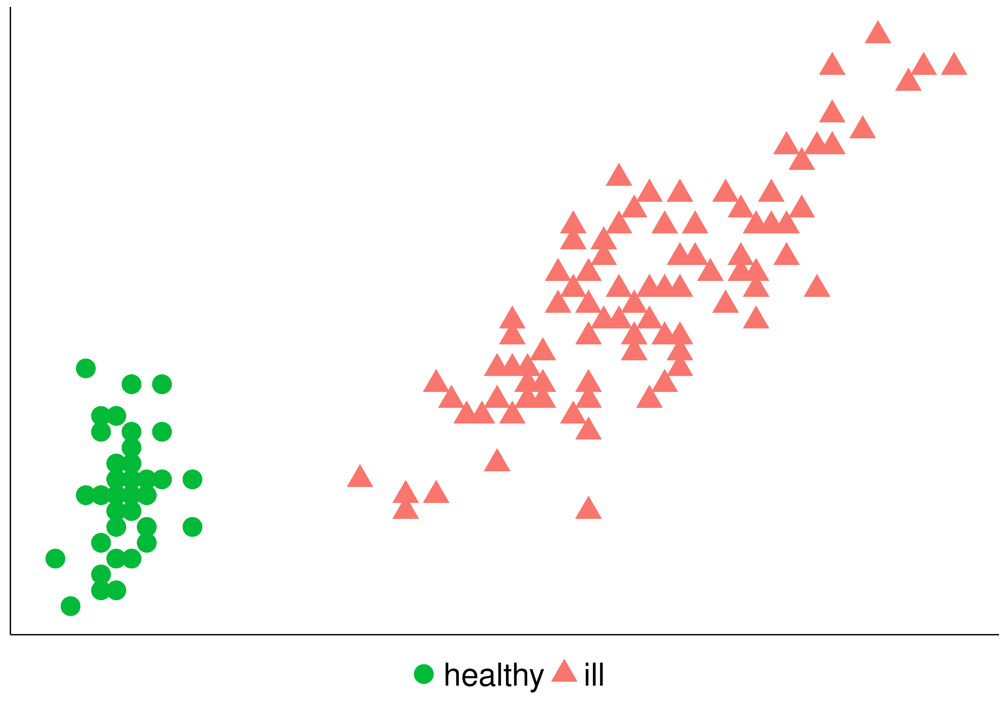 |
 |
How to treat ordinal problems
One way to tackle ordinal problems is to transform the problem into other simpler problems. As presented in Ordinal Regression Methods: Survey and Experimental Study, these are some common ways:
- Naïve approaches
- Regression
- Nominal Classification
- Cost-sensitive classification
- Binary decomposition
- One vs All
- One vs One
- Threshold models
- Proportional Odds Models
The interested reader can find these approaches explained in more detail in the linked paper. As this is not the point of the post, it only merits mentioning what the common ways to treat the problem. In this work we use a different and mixed approach, the use of unimodal probability distributions and ordinal loss functions.
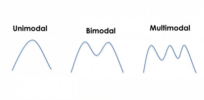
Unimodal distributions
So, what’s an unimodal distribution?, you might wonder. It’s a probability distribution that, as the name implies, only has one mode. Simply put it means that it has one single value that repeats the most often. In the figure bellow it’s the distribution to the left. The other distributions have two and three values which are the most common respectively.
As we want to approximate the logical reasoning of what a person would think when looking at a picture the best option is to force the output of the DNN to be a unimodal probability distribution. As you can imagine, the distance between classes is very important because nobody would mistake the picture of a baby with a grown man with a beard, right? It would make sense to mistake a baby with a toddler, or a grown man with a young adult or an older person, but not two ages that different. So when using unimodal probabilities distributions you’re taking the prediction of the net and making the probability for each class descend as it gets further from the predicted one.
The following probability distributions were used:
- Binomial
- Poisson
- Chi-squared
- Student’s t
Only the first distribution, Binomial, improved the baseline consistently and was clearly better than the other distributions, so that was the one included in the final study.
Evaluation Metrics
Accuracy:
It’s the most common and simplest way to measure the performance of a classifier when predicting new instances. It’s as simple as the rate of correctly classified samples, namely:
Accuracy = (Number of instances correctly predicted) / (Number of total instances).
It’s easy to calculate, but can be deceitful when the data is imbalanced, which causes many problems.
Top-k Accuracy:
This is the same as the normal accuracy but if the correct class is among the first k predicted classes, it’s considered as a correct prediction. It’s typically used in problems with a huge number of classes. For this metric to be usable with a classification model, the model has to output a probability for each class to order the predictions.
In this case it makes sense as an ordinal classification metric because we’re also using unimodal distributions at the end of our DNN.
Quadratic Weighted Kappa:
It’s a modified version of the Cohen’s Kappa statistic with weighting. In this case we use a quadratic weighting system, which means that the weights increase as the quadratic of the distance among classes increases. It’s the best metric to compare the performance on a ordinal dataset as it truly takes into account the magnitude of the error. For further reading this post on Kaggle explains it very well.
Deep Learning for Ordinal Classification
As mentioned earlier the approach taken in this work was novel because it used two different methods to account for ordinality during training: first, a layer at the end of the ResNet was added to shape the output to a unimodal distribution; and secondly, because new loss functions were implemented and used during training to account for the distances or magnitude in the class errors.
Ordinal Loss Functions
The point of training DNNs with a gradient descent algorithm is to modify the weights of the network during training to correct the errors made when predicting the class of new instances. To improve a DNN in a ordinal problem the best bet is to take into account the distance between the predicted class in training and the ground truth. This is done with a loss function that calculates the error across multiple instances (batch) and propagates the error backwards into the weights of the network to modify them according to the amount of error. It’s here that we can best take into account the distance of classes and correct the network in direct relation to the distance of the error.
To achieve this we have to use functions that calculate the distance between probability distributions, as we want to turn the output distribution of the network into the ideal distribution, namely a probability of 1 for the real class and 0 for the rest. The most common loss function used, the cross entropy loss function, doesn’t take into account the shape of the distribution meaning that different distributions could have the same loss value.
The loss functions used were:
- Quadratic Weighted Kappa (QWK): proposed as a loss function in this article
- Earth Mover’s Distance (EMD): measure of the distance between two probability distributions, find more on wikipedia. Proposed as a loss function in this article.
- MSE: this is a novel proposition from this work. Two versions were used:
- wMSE: uses linear weights to penalize the distance between classes
- qMSE: uses quadratic weights to penalize distance between classes
Experimental Results
I’ll spare you all the details from the experimental setup, the data partitions, data augmentation, the training parameters, the residual architecture, the convergence graphics and whatnot, and I’ll go directly to the results.
For the comparison of the performance of the different methods we used a baseline model, a ResNet without any ordinal modification that treats the problem as a normal classification (also called nominal classification) problem, and five different combinations of ordinal models. One ordinal model (2) doesn’t use an ordinal loss function, it only uses a binomial distribution for it’s output. The rest (3-6) use both methods. So the configurations used are:
- Baseline, loss: cross entropy
- Binomial, loss: cross entropy
- Binomial, loss: EMD
- Binomial, loss: wMSE
- Binomial, loss: QWK
- Binomial, loss: qMSE
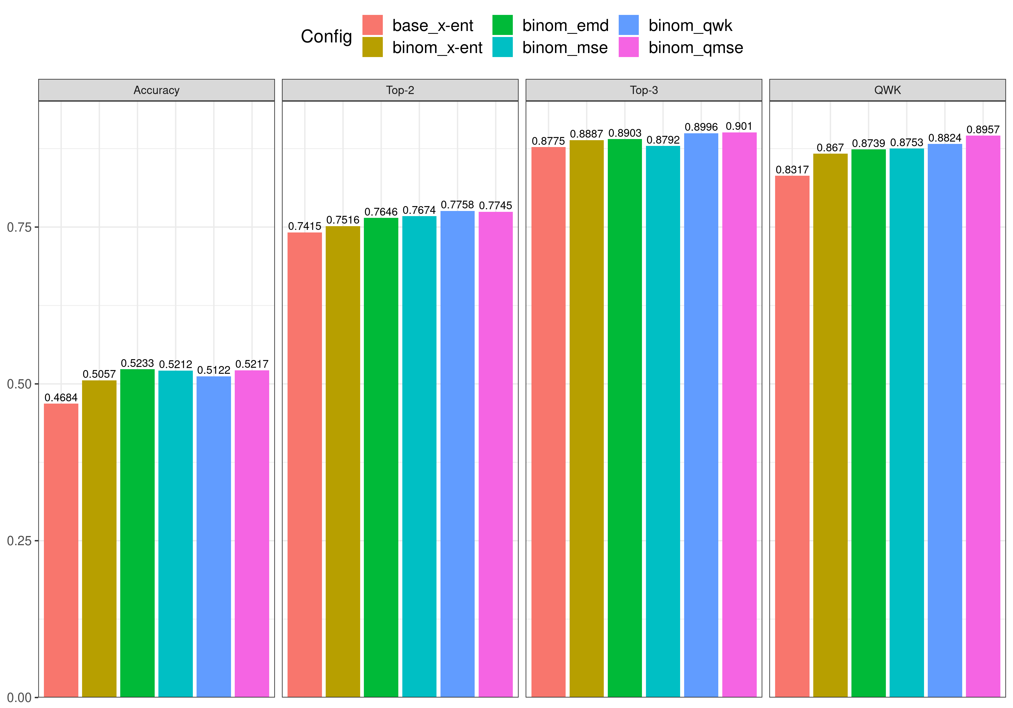
The metrics for the predictions on the test set for each of the models are included in the next table. The rows correspond to each of the elements in the previous list, and the columns are the values for each evaluation metric. The values in bold are the best achieved for each metric.
| Configuration | Accuracy | Top-2 | Top-3 | QWK |
|---|---|---|---|---|
| base (x-ent) | 0.4684 | 0.7415 | 0.8775 | 0.8317 |
| binom (x-ent) | 0.5057 | 0.7516 | 0.8887 | 0.867 |
| binom (emd) | 0.5233 | 0.7646 | 0.8903 | 0.8739 |
| binom (mse) | 0.5212 | 0.7674 | 0.8792 | 0.8753 |
| binom (qwk) | 0.5122 | 0.7758 | 0.8996 | 0.8824 |
| binom (qmse) | 0.5217 | 0.7745 | 0.9010 | 0.8957 |
The same data of the table but plotted on a barplot is shown bellow. We can learn many things from this plot. It can be seen that (logically) increasing the k parameter in Top-k Accuracy makes the models achieve higher values of accuracy, but it doesn’t seem to reflect the performance of the ordinal models with unimodal probability distributions on their output, because the baseline model also achieves higher values, so an intrinsic ordinal metric is required, like Quadratic Weighted Kappa. As it can be seen in the right most figure, with this metric there’s a greater difference between the ordinal models and the (nominal) baseline model. The best result is obtained by the model with the quadratic weighted MSE loss function, binom_qmse, followed by the one that used QWK as the loss function, binom_qwk.
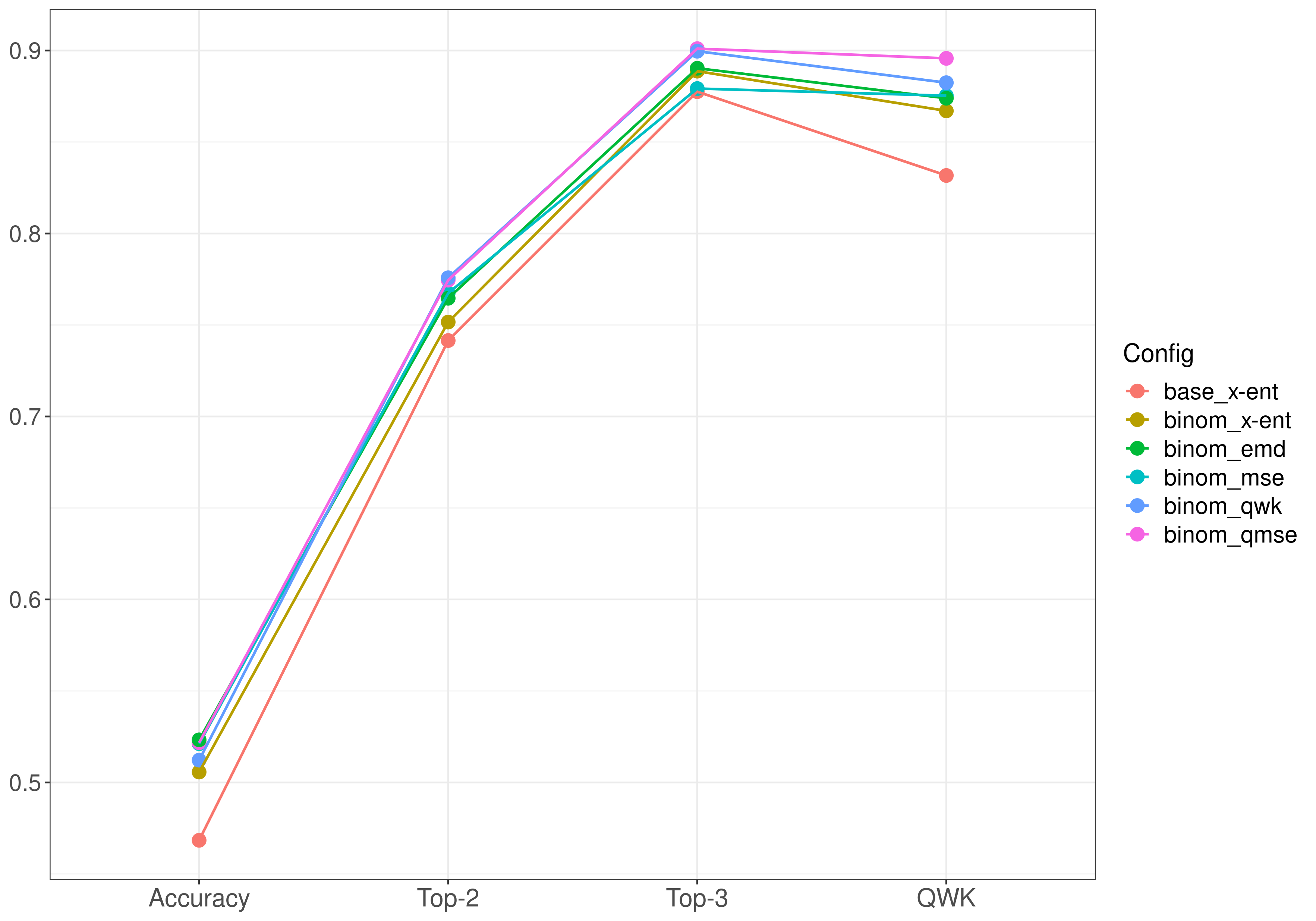
The differences in the scores shown in the previous comparison are easier to see in the following figure. Here, on the horizontal axis the same metrics shown previously are included, but we have continuity among models, which are shown across metrics with the same color. So, each line represents a model configuration and the dots the score for each metric. Here we can see that the baseline model (base_x-ent), trained with cross entropy, under performs on all metrics with respect to the other models that have some kind of ordinality. In the non-ordinal metrics this difference is not very big, but it increases when using QWK as a metric. The second worse model, binom (x-ent), is the model with the binomial output and without an ordinal loss function, namely, it uses cross entropy as a loss function. From this we can reason that the models that worked the best were the ones with an unimodal probability distribution and an ordinal loss function. The one that obtained the best results across all metrics is almost consistently binom_qmse, which clearly outperforms the other ordinal models. The second best model, binom_qwk, also seem to be consistently the second best across all metrics. It’s also worthy of mention that the inclusion of quadratic weights for the MSE loss function, binom_qmse, significantly outperforms the linear weighted version, binom_mse, and that this version scores the same QWK value as binom_emd, which previously existed in the literature.
In the following three figures the difference between evaluating the training process with a non-ordinal and an ordinal metric can be seen. The first two figures, (a) and (b), show the evaluation metrics, Accuracy and QWK, during the training process, and the third one (c) shows the values for QWK on the validation partition (also during training). In the accuracy figure (a) the baseline model (trained with cross entropy loss) starts to score better values of Accuracy than the rest of the models early on, approximately in epoch 20. This same training, when evaluated with a ordinal metric, QWK (b), paints a very different picture. The baseline model takes longer to converge than the rest of the models, and in the end appears to beat most of them, but in reality, if we watch the QWK validation plot (c) it turns out that it’s overfitting, as its values end as the worst in the validation partition.
| Train Accuracy | Train QWK | Validation QWK |
|---|---|---|
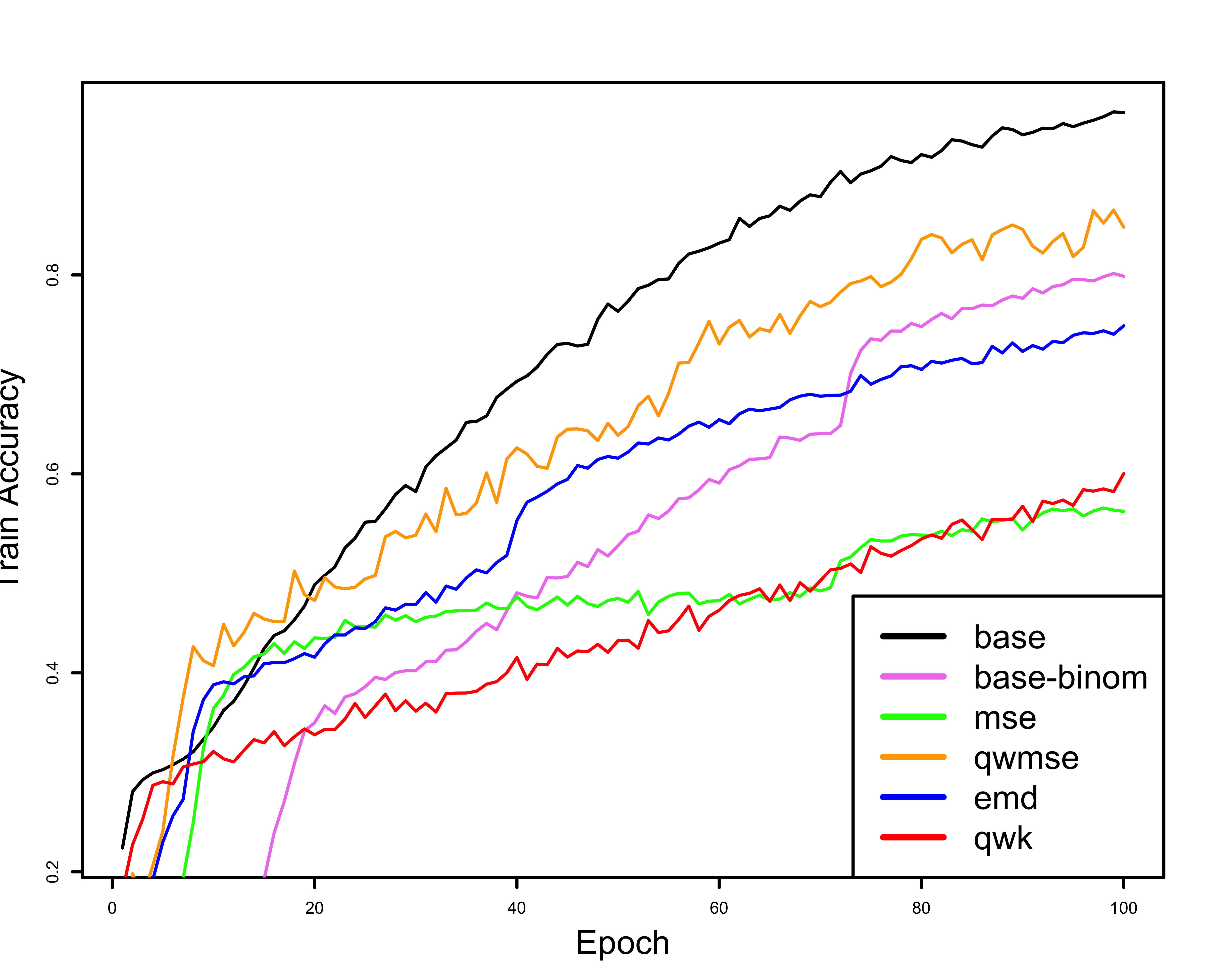 |
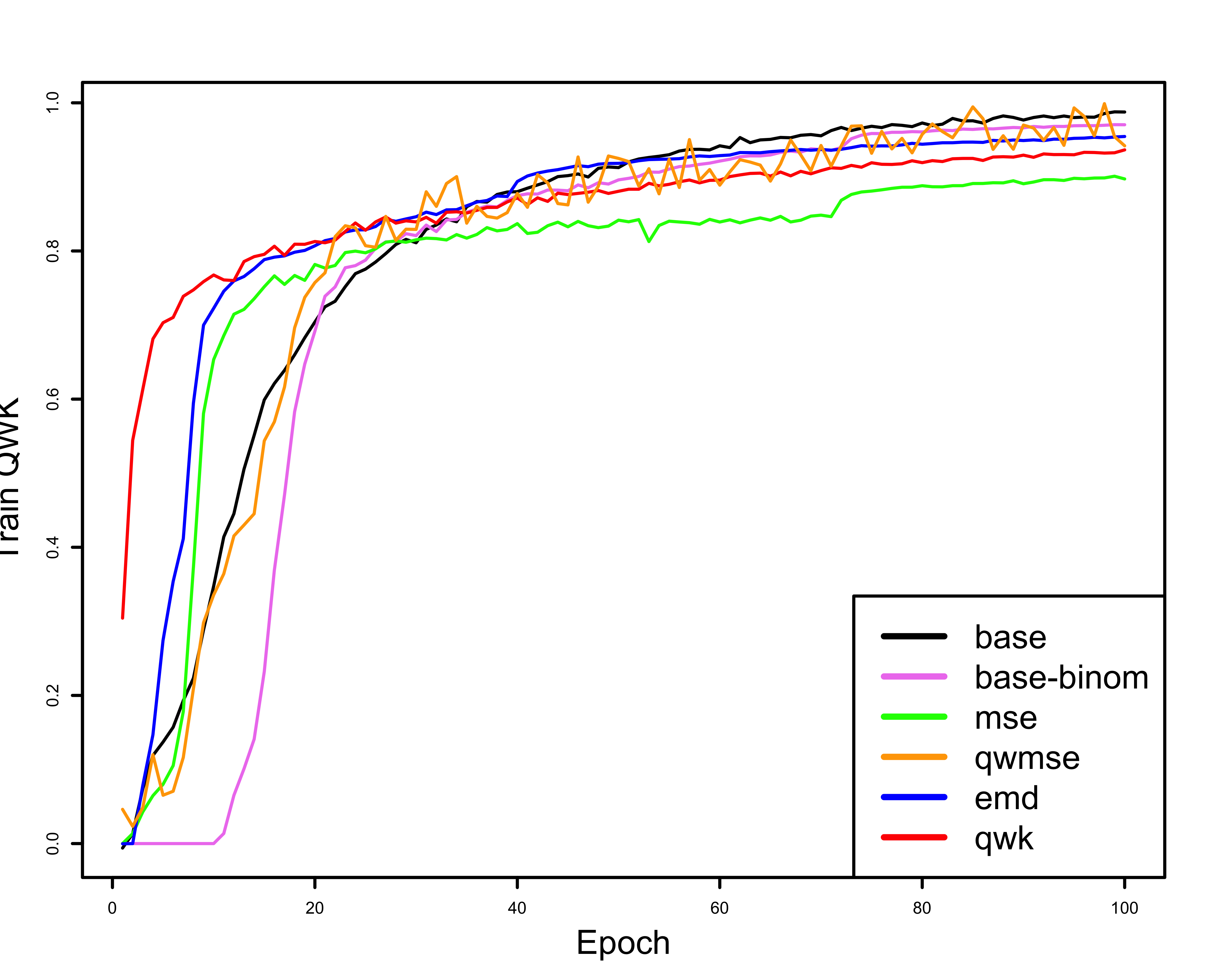 |
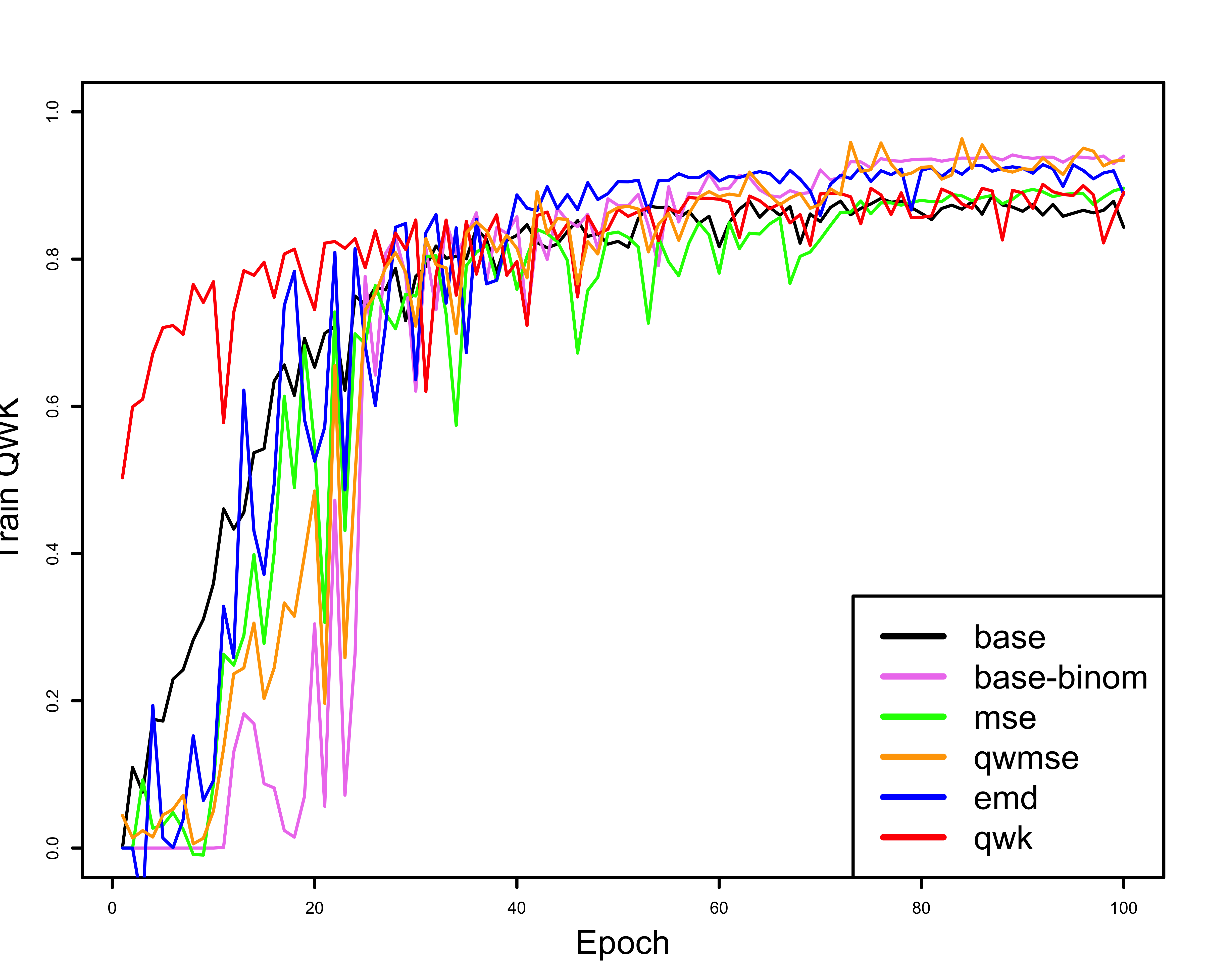 |
| (a) | (b) | (c) |
I think it’s also interesting and important to mention that in figures (b) and (c), which use QWK as a metric, the model using the QWK loss function starts scoring very high values, much higher than the rest for a few epochs. This is the case because the model is being trained on the same metric that it is being evaluated on, so it kind of has a head start, but in the end it doesn’t hinder the training process, as seen in the figures and tables that show the test results, where it’s almost always the second best method.
Conclusions
With the results obtained and shown in the previous section, it can be seen that when working with ordinal classification problems, using models adapted to consider the ordinality in the data, both in it’s output probability distribution and during the training process with ordinal loss functions, increases notably the performance of a baseline model that treats the problem without taking into consideration the ordinal nature of the data. It can also be seen that using ordinal loss functions prevents overfitting during training, and the need to use the proper metrics to evaluate the underlying problem. Using the proper evaluation metrics when using datasets with an ordinal nature is as important as using metrics to take into consideration underrepresented classes in imbalanced problems, where one may end up with an accuracy of 95% or higher while completely omitting imbalanced classes.
It is worth pointing out that this area of classification is often rarely used outside of academia, even when achieving noteworthy improvements. When treating ordinal problems as nominal classification, an important and intrinsic part of the information included in the data is being omitted, so correctly using all the available information is crucial to improve the predictions. If ordinal classification is often rarely used outside of academia, the usage with Deep Learning model is even rarer, and surely requires future work to improve on this area.
The End
That’s it. Thanks for making it this far!